Transmission Line Terminations Techniques For PCB

Signals propagating down a trace reflect off the far end and travel back toward the source. These reflections can cause noise, and therefore signal integrity problems.

These reflections can be controlled if we design our traces to look like transmission lines. Then, for “long” traces (those longer than the critical length) we can control reflections using transmission line termination techniques.

Transmission Line and signal reflection

The ideal model of a transmission line is one that is infinitely long. If we take just a portion of that line, and terminate it in its characteristic impedance, it still looks infinitely long when viewed from the front (Figure 1). And, there is no reflection from the far end.

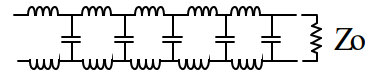
Figure 1 :If we terminate a portion of a transmission line in its characteristic impedance, it still looks
infinitely long.

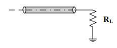
If we terminate a transmission line in anything other than its characteristic impedance, a reflection will occur. The magnitude of that reflection can be determined from reflection coefficient.

The reflection coefficient, is calculated as:

Reflection coefficient = (RL – Z0)/(RL+Z0)

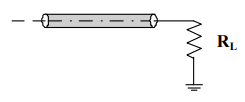
Where RL, the load resistor, and Zo, the characteristic impedance of the transmission line, are as shown in Figure 2.

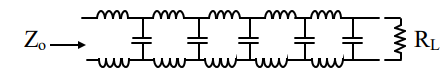
Figure 2: The magnitude of the reflection is determined by the relationship between RL and Zo.

Reflection coefficient has a value between –1 and +1

If the trace is left open circuited, the reflection coefficient is +1 and there will be a 100% reflection back toward the Driver.

If the trace is shorted, the reflection coefficient is –1 and there will be a 100% reflection of the opposite sign back toward the driver.

If the line is terminated with a resistor whose value is the same as the characteristic impedance of the trace (Zo), then reflection coefficient is zero and there will be no reflection at all.

If a reflection does occur, and propagates back to the driver (source), it can reflect again off the source. If that output impedance of Driver is exactly equal to   Zo, then there will be no further reflection from the source.

If the output impedance of the driver is different than Zo, an additional reflection will occur. The magnitude of that reflection is again determined by a reflection coefficient.

The reflection coefficient, is calculated as:

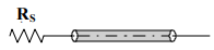
Reflection coefficient = (Rs – Z0)/(Rs+Z0)

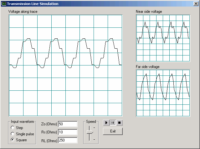
Transmission Line Simulator example

There are five common termination techniques seen in typical circuits. Termination strategies can be effective in eliminating, or at least minimizing, transmission line reflections. But no individual strategy is perfect. Each one has a tradeoff of some type.

Parallel Termination:

Parallel termination is most intuitive and possibly the most common. It simply consists of a single resistor from the trace to ground or to Vcc.

This technique has several advantages:

(1) the value of the resistor is relatively easy to determine

(2) there is only a single component

(3) it is easily connected, and

(4) it performs well with distributed loads (i.e. loads that are distributed along the trace.)

There is only one drawback to this type of termination:

It provides a continuous DC path to ground. Therefore, continuous DC current can flow through it at all times. This may or may not be an issue for a single trace.

But if your design has a thousand or so impedance-controlled nets, the total power dissipation in a thousand terminating resistors can become quite significant!

Thevenin Termination:–

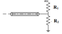
A closely related variation of the parallel termination strategy is the Thevenin termination. This consists of a pair of resistors, one going to ground and other one going to Vcc. The pair of resistors provide a pull-up/pull-down function as well as a termination function. Therefore, it can improve noise margins in certain situations, and performs as well as the parallel termination with distributed loads. The parallel combination of the two resistors must be Zo, or:

Z0 = 1/(1/R1 + 1R2)

The optimum values for R1 and R2 primarily optimize (minimize) the power dissipated in the circuit. This optimum value can be difficult to determine. Other drawbacks to this strategy include the addition of an additional component, and the fact that DC current still flows through the resistor pair at all times. And this strategy is only well suited for bipolar (two-state) devices, not for tri-state logic families.

Note that there are different currents flowing between Vcc and Gnd, through R1 and R2, depending on the logic state. And this current changes at the same rate (di/dt) as the logic state changes (the rise/fall time of the signal).

In this respect, the two resistors look exactly like a switching logic gate. Therefore, they might need to be decoupled (with bypass capacitors) just as a logic gate might need to be decoupled (with bypass capacitors) to minimize EMI.

AC Termination:–

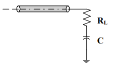
AC termination is the addition of a capacitor in series with the parallel terminating resistor. The primary advantage of this is that the capacitor blocks DC current, so there is no steady-state current flowing through the termination. At first glance it would appear that this strategy otherwise has all the advantages of the parallel termination strategy. However, the “cost” of this, of course, is the added component.

If a large capacitor value is used, there can be considerable power dissipation.

 If a very small capacitor is used, it will cause overshoot and may interfere with the rise and fall times of the signal. As the voltage across the terminating resistor changes, the current through the capacitor changes. This causes the capacitor to charge or discharge with an RC time constant related to the component values.

If the time constant is too short, the capacitor charges during the half-cycle and the voltage at the receiver changes accordingly.

AC Termination – simulation with 50 ohm and 2nF capacitor

Simulation results shows that with a relatively large capacitor of .002uF with a resistor of 50 ohm the waveforms look very clean.

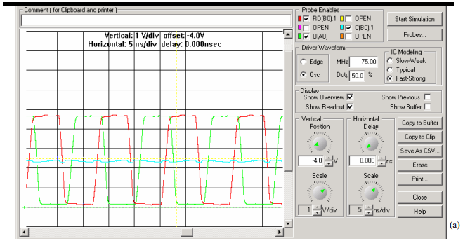
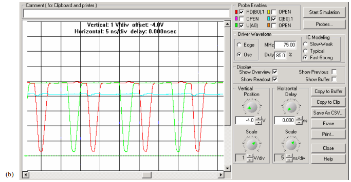
AC Termination – Simulation with  50 ohm and 200pF capacitor

Simulation result shows that there is overshoot and undershoot in the receiver waveform.

Each transition of the driver signal is followed 5 ns later with the same (magnitude) transition at the receiver. But then the receiver voltage continues to rise (or fall, as the case may be) as the capacitor charges and discharges.

If this over/undershoot is severe enough, logic errors may result. As is seen, the driver signal is still relatively clean. In extreme cases the voltage at the driver may also start to change.

Note that this is not a reflection or a impedance matching issue but it is changing reference voltage that shifts the value of the waveform at the receiver.

The line has an intrinsic capacitance (Co) and an intrinsic inductance (Lo) that is expressed in units per unit length. In absolute terms, the values increase with increasing line length. At some point the values become large enough that ringing occurs as the average value across the capacitor changes.

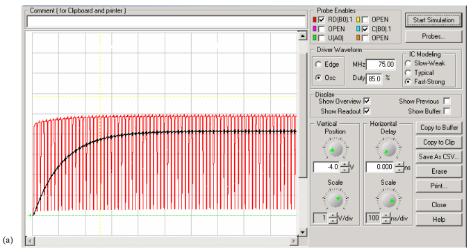
Case1 : simulation ofRising waveform terminated correctly 5 ns long line with a large (.002 uF ) capacitor

The voltage across the capacitor (black line ) rises in a controlled manner to 50% of the voltage at the receiver (red line).

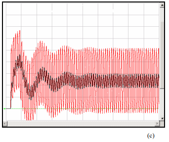
Case 2 : simulation of 5 ns long line with a smaller, 200 pF capacitor.

Note that there is a short stabilization time, but then the system settles down.

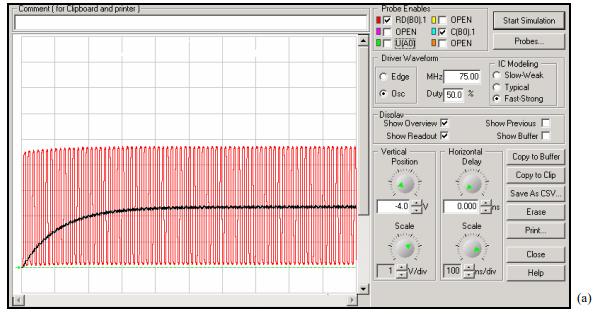
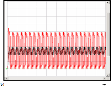
Case 3  : Simulation of 30 ns long line with a smaller, 200 pF capacitor

Note that The value of the capacitor interacts with the parameters of the transmission line to cause oscillations that take a finite time to die out.

Admittedly 30 ns line length might be an extreme example from a PCB standpoint. But it may not be extreme if we are talking about transmission lines that connect two pieces of equipment separated by some distance.

Case 4 : effect of duty cycle

If we have a uniform bit-stream (50% duty cycle) traveling down a trace, the capacitor will charge to the average value between a logical zero and a logical one

If the duty cycle changes, that voltage level will adjust to a new average value.  With 85% duty cycle The voltage across the capacitor rises to a higher level, but the waveforms themselves are still clean and undistorted.

Ac Termination – Simulation with 85% Duty cycle

Ac Termination – Simulation with 85% Duty cycle

In conclusion AC termination can be effective (Performs as well as parallel without the dc power drain) but C is difficult to optimize and Can lead to timing problems

If the capacitor is too large, the benefits (of blocking the DC component of the signal) may be reduced.

Long lines may introduce unexpected oscillations when the average DC voltage component of the signal changes.

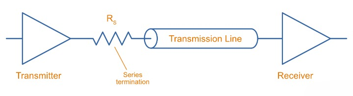
Series Termination:

Series termination is becoming more and more common in today’s high-speed designs. It has the two desirable attributes of a single component and no DC current draw at all.

Series termination resistor is placed at the front of the trace, not the end; the end is left open-circuited. Therefore, there is a 100% positive reflection from the far end of the trace that reflects back towards the front.

The value for the series termination resistor is set so that the sum of termination resistor value and the output impedance of the driver totals to the impedance of the trace. That way, there is no secondary reflection from the driver.

The voltage pattern we expect to see is a single, positive reflection from the far end of the trace which travels to the front of the trace and is completely absorbed in the source resistor and driver.

That means that we have to know the output impedance of the driver. Which is generally specified by the manufacturer in datasheet. But an additional complication is that the output impedance is often different depending on the output state.

Below simulation illustrates a series termination simulation where Driver has a logical high output impedance of approximately 19 Ohms and a logical low output impedance of about 5 Ohms.

Simulation results (a) and (b) are for termination resistor values of 31 Ohms and 45 Ohms, respectively.

Note how the rising waveform in (a) and the falling waveform in (b) appear to be terminated correctly. But both the rising and falling edges cannot be terminated correctly at the same time!

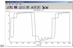
Rising waveform terminated correctly

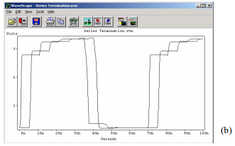
Falling waveform terminated correctly

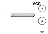
Diode Termination:

This termination strategy is really just a reflection limiting strategy. No attempt is made to absorb reflections or to prevent them. The intent is to let them occur and simply limit them to one diode drop above Vcc a(a) and (b) one diode drop below Gnd.

Diode Termination Does not depend on Zo, it can Can be placed anywhere on line and adds to Little increase in power.

Transmission line termination strategy summary

• Pros:
  • Performs as well as parallel without the dc power drain
• Cons:
  • C is difficult to optimize
  • Requires 2 components
  • Can lead to timing problems

• Pros:
  • One component No dc load
• Cons:
  • Can be difficult to optimize
  • RS There IS a reverse reflection.

• Pros:
  • Does not depend on
  • Zo Little increase in power
  • Can be placed anywhere on line
• Cons:
  • Reflections still exist Requires 2 devices
  • Diodes must be FAST with low foreword voltage

Contact Us: info@sysargus.com

Learning Platform for Product Engineering professionals imparting guidance and sharing knowledge on Electronics System Design Best Practices.

Connect with us:-